Vítejte!

If you are faced with the task of implementing and performing vibration diagnostics in your company, then do not panic. This area offers both simple and complex procedures and methods. You will start with the simplest ones and gradually work your way up to more complex ones. At the beginning, you will perform measurements very similar to those made with a voltmeter. Only you will not measure voltage, current or resistance, but vibration values.

The basic task of diagnostics is to prevent unexpected failures, because eliminating their consequences entails high costs. If a rolling bearing breaks down unexpectedly, then other machine components around it will also be damaged. That is why the repair is very expensive.

Diagnostics will warn you in advance of the worsening condition of the bearing, you can plan a replacement during a regular shutdown and the costs will be much lower. The task of diagnostics is therefore to reduce maintenance costs.

In the past, machines ran until they broke down. Then they were repaired. This approach had two basic disadvantages. Let's imagine a relatively small problem, for example bearing wear down. Replacing of the bearing would be easy and quick. However, if the wear is great, then the bearing breaks down and the entire rotor stops rotating. The rotor weight is several hundred kilograms. It does not stop easily. There is enormous inertia present, which can destroy the entire machine in a few seconds. Then the repair is long and expensive.

Another disadvantage is the sudden stop of the production line, again due to the wear of one bearing. For example, the line produces products worth a million in 1 hour. If the repair takes several hours, then there will be a loss of several million.

The subsequent development of the maintenance system then reached the stage of preventive replacements. Every component that wears out over time was replaced at defined time intervals. Let us list the basic disadvantages.

• Maintenance costs are high because something is replaced all the time.
• Secondly, in most cases, it is replaced unnecessarily because the component is still in good condition.
• And thirdly every maintenance intervention is not completely perfect. For example, the installation of a new bearing can be performed poorly and the condition of the new bearing will deteriorate quickly, so that eventually an unexpected failure will occur anyway.

Subsequently, another maintenance system appeared, which is the predictive maintenance. The condition and wear out of the machine are measured regularly, and if it is getting worse, then maintenance intervention comes. That means, only when it is really needed.

But what methods can be used to measure the condition of the machine?

Vibration diagnostics has an absolutely dominant role in measuring the condition of the machine. It can accurately measure the severity of all basic machine failures. In the following chapters, we will explain everything that is needed for its use. We will not go into theoretical details and mathematical formulas. This is not necessary for the successful implementation of vibration measurements and the subsequent evaluation of the machine condition.

In the past, acceptable vibration was tested by putting a coin on a machine. If it fell, the vibration was considered high.

There are many other ways to measure machine condition, but they are very specialized and very narrowly focused. None of them achieves the performance of vibration diagnostics.

What will we need? First of all, a measuring device, let's call it a vibration analyzer, a vibration sensor and a cable to connect the sensor to the device. Equipped like this, we go to the machines, we call this a route. We will perform measurements on each machine, which will be saved in the device's memory. After returning from the route, we will transfer the measured data to a computer and evaluate them.

To perform vibration diagnostics, we use a program supplied by the manufacturer of the vibration analyzer. We will create a list of machines and the measured data will be saved to them.

We will go to the route at regular intervals, the more often the better. Of course, we cannot go every day. The optimal interval is about 2 weeks. If we have machines whose operation is essential for the entire factory, then it is better to use online systems that measure continuously.

Now we have the data in the computer and it needs to be evaluated. This means determining the current machines condition and, if necessary, planning repairs or adjustments. How do we do this? There are several ways to look at the measured values.

If any standard exists, then it can be used. The standard will tell us the values of vibration limits. Usually, the warning and danger limits. If the warning limit is exceeded, the machine can still be operated, but we should plan a maintenance intervention as soon as possible. Exceeding the danger limit means the machine must be shut down immediately and repaired. The basic standard is ISO 20816.

Then other procedures are needed.

If we have several identical or similar machines, then we can compare the values between them. If the vibrations on five of six identical machines have a value of 2 and on the sixth the value is 8, then there is clearly something wrong with the sixth machine.

Another option is to analyze the trend of the development of vibration values. If the trend is stable over the long time, then the operating condition is also stable. If the vibration values increase, then some damage is increasing and the machine needs to be repaired or adjusted.

The trend or comparison with values from the past is the best way how to evaluate the machine condition. When we can see even a small increase; this means that the deterioration of the condition is only small and we have enough time to plan a maintenance intervention.

It is the same with vibration diagnostics. It will never be 100% successful. Sometimes the fault is too hidden inside the machine and may not be easy to find it in the vibrations. Or its development was very quick and during the last route everything was still fine.

Suddenly an unexpected break occurs. Then the warning and danger limits need to be reduced. So even an unexpected break can have a positive meaning for the future.

Vibration diagnostics is absolutely essential in taking care of the condition of machines. There is no other type of diagnostics that can find such a wide range of faults and wear.

Vibrations are the oscillating, repeated movement of mass between two extreme positions. The important is whether the amplitude of the vibrations (it means the distance between the extreme positions) is acceptable for the machine operation. The velocity of the oscillating movement is also important.

A spring and a mass hanging on it is a good example for understanding vibrations and their properties. If we stretch and release the spring, the mass will start to oscillate up and down. The oscillation will decrease due to air resistance and internal friction of the spring until it stops completely. Let‘s imagine that these influences do not exist and the oscillation does not decrease. We can attach a pen to the mass and put a strip of paper behind it. Now we stretch and release the spring and at the same time we start to move the strip of paper to the left. The pen will draw a curve. This curve shape of the vibrations is a basic shape and mathematically corresponds to the sine function. We will call the recording on the paper as a time signal of vibrations and we can evaluate other useful vibration parameters from it.

The amplitude of the vibration can be easily measured using the 0-P amplitude. We call it the peak value and it is the distance from the mean value of the signal (which corresponds to the rest position of the weight) to the maximum value. In the figure, the 0-P amplitude is equal to the number 5.

For completeness, we should mention the P-P (Peak-Peak) value, which is the distance between the maximum and minimum values. For a symmetrical signal shape, the P-P value is twice the 0-P value. But many signals are asymmetrical and this relationship is not true.

The task of digitization is to convert an analog signal into numbers. The picture shows just an example of a few values read from the signal. We select a time and read the value. We will call it as the sample at defined time. This is just an example of reading.

First of all, we need to read values at regular (equal) time intervals. For example, the interval between readings will be 1 ms (1ms = 0.001sec). If the signal length is, for example, 1 sec, then we will get 1000 samples, it is a series of 1000 numbers. In the future, we will always call individual readings in a time signal as samples. If we have enough samples, then we can apply various mathematical formulas to them and we can calculate other diverse results.

So far, we can measure the amplitude of time signal as 0-P or P-P values. The amplitude of time signal can also be measured as the average value of all measured samples. The average value is calculated as the sum of the values of all samples and divided by their number. It is the same as the average weight of one apple in a basket. We add up the weights of all apples together and divide the sum by their number.

Now we will try to add up all the values of the samples in time signal and divide by the number. But it is not useful. The sine signal is symmetrical around zero, then the average value will be zero. We must do something differently.

The solution is to convert the signal waveform only into the positive half. We will achieve this by working with the absolute values of the samples. It converts negative values into positive ones, e.g. the absolute value of -3 is +3. The absolute value of +3 remains +3, nothing changes here.

The new shape of signal is in the image.

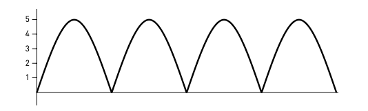
If we calculate the average AVG value of the signal from the figure above, we get 3.2. For the sine function, the average AVG value is always equal to 0.64 multiplied by the 0-P value. In the image, the 0-P is equal to 5 and the average is 0.64 x 5 = 3.2.

!!! Attention! We must not apply this conversion to signals which do not have the shape of a sine function.

For the curious readers, we also present the mathematical formula for a continuous signal waveform, which we will denote as f(x)

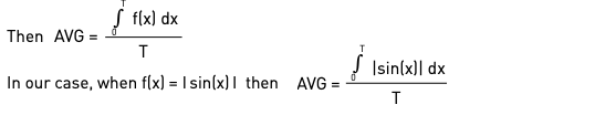
Let‘s fill in and measure the area under the sine function. Mathematically, this is the calculation of a definite integral, as we mentioned above. Now we will draw a signal whose samples all have the same value. The area under the signal is calculated as the length multiplied by this sample value. It is the area of the rectangle. Our task is to find such a value that the areas of both signals are identical.

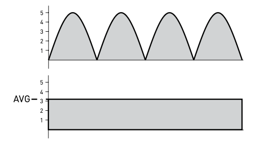
This desired value will be equal to 3.2 (0.64 * 5). I just want to remind you again. This conversion is not valid for signals that do not have the shape of a sine function.

Let‘s go back to the example with apples. For example, we have 20 of them with different weights and their total weight is 4kg. The average weight is 4kg/20=200g. If we take 20 apples, each with an average weight of 200g, then together they will also weigh 4kg. This is the same approach as replacing the sinusoidal (irregular) waveform with just a signal where all amplitudes are equal to the average value. So, it is a straight line.

We will explain it with the following examples.

We have already described the case of a sinusoidal waveform. The average value is equal to the value 0-P multiplied by 0.64

When we calculate the average value from a rectangular waveform, then after converting to an absolute value we see almost the same as after converting to a rectangle. It follows that the average value AVG is almost the same (only slightly smaller) as the value of 0-P.

If the signal contains only shocks, the situation is the opposite. The area inside the pulses is small, and thus the height of the rectangle for deriving the average AVG value is small.

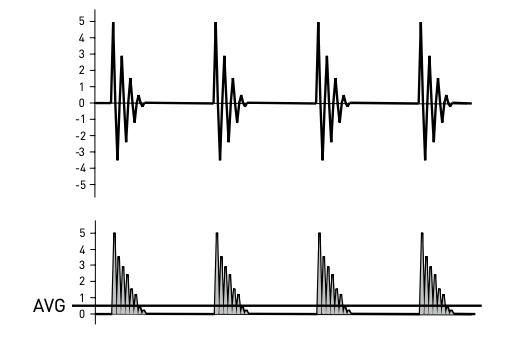
We have shown that there is no fixed relationship between the average and peak values.

The average value would work well as an indicator of the size of vibrations, but it is not used in practice. A similar value is used, which we call RMS (Root Mean Square).

Its advantage is that it corresponds to the energy contained in the signal. Let‘s imagine the level of the force that subsequently causes vibrations under the concept of energy.

For example, in case of unbalance, it is the centrifugal force that brings us problems because it shakes the entire machine, strains the fastening screws, and puts a load on the bearings. Therefore, we try to reduce the size of the force as much as possible. And this is equivalent to trying to reduce vibrations. If we reduce vibrations, we have reduced the force acting on the machine.

How is RMS calculated? It is similar to the average value, only all signal samples are squared first. This simultaneously achieves their transformation into positive values. Then the square root of the average value is calculated.

In the figure we see the signal sin2 . The maximum amplitude has increased to 25. This corresponds to 52 , when the maximum value was 5 in the original signal. Then we calculate the average value and take the square root of it.

If the waveform of the signal corresponds to the sine function, then the RMS value is equal to the peak value 0-P multiplied by 0.71. With a peak value of 5, we get RMS=3.55. This can be expressed again as a constant signal (rectangle) with a height of 3.55 and a width equal to the duration of the signal.

I would like to remind you again that the conversion constant 0.71 can be applied only to a sinusoidal waveform. The explanation is the same as we showed for the average value.

A little bit of math

Let us have a digitized signal y. That is, we have a sequence of samples

we have N sample values.

For curious readers, I will just add the information, that both the AVG and RMS values do not depend on the duration of the signal. In other words, a longer signal will not give us larger values. The reason is clear. These are average values (we divide by the number of samples N). If the signal has more samples, then their sum will be larger, but after dividing by the number of samples we will get the same value as for a shorter signal. RMS and AVG values will be stable for both signals. For machines with speeds above 10 Hz (600 RPM), it is enough to measure a signal with a length of 1 second. For low-speed machines, we measure longer. The signal should contain at least 10 revolutions. This means that at a speed of 2 Hz we measure at least 5 seconds (one revolution lasts 0.5 seconds).

Different spring stiffness and different mass affect both the amplitude and frequency of the vibrations. Frequency is how many periods of up and down movement the mass makes in a given time, usually 1 second.

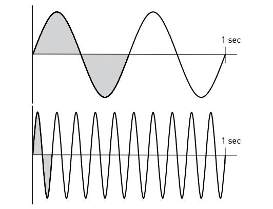
In the picture, we can see two time signals. Both lengths are 1sec. The mass above has reached the minimum and the maximum position twice within 1sec. Below, the movement of the mass was faster and reached the minimum and the maximum ten times. It is clear that the mass keeps repeating the up and down motion. What is the basic (shortest time) motion which is repeated periodically? This basic movement of up and down is filled in the figure. We call its length as a period. Since the entire recording takes 1 sec, the period of the slower vibration at the top takes 500ms. The period of the faster vibration at the bottom takes 100ms.

The frequency is calculated in Hz and tells us how many times in one second the periodic motion repeats. In our example above, the frequency is equal to 2 Hz (2 times the period) and below it is 10 Hz (10 times the period). If we denote the length of the period by T, then the frequency:

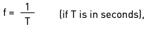
or alternatively:

Even the speed (rotation) is a repetitive motion, where the basic period is one rotation of the shaft. The rotational frequency can also be expressed in Hz, which is the number of rotations per 1sec. We will call the rotational frequency a speed frequency or just speed

It is more common to measure in RPM. This value indicates how many times the shaft turns in one minute. The conversion is obvious:

The number is 60 because a minute has 60 seconds.

A vibration sensor is a device which converts vibrations into an electrical signal

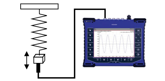
The picture shows the sensor attached to the mass. If the mass vibrates, an electrical signal appears at the output of the sensor and we measure it in the analyzer. The instrument then shows the vibration waveform, just the same waveform as we drew on paper before.

Analogy with alternating voltage in the electrical network

It is similar to measuring the voltage in the network. It also has an amplitude whose RMS value is 230 V – in the US it is 110 V.

In the electrical network, the voltage has a waveform corresponding to the sine function, so we can already calculate that the 0-P value in the network is 230/0.71=324 V or 110/0.71=155 V.

The frequency of the network is 50 Hz or 60 Hz in the US, it means the length of one period is 20ms or 16.7ms.

We have already explained the frequency. What is the importance of frequency for machine diagnostics? It is essential. Different faults are manifested in vibrations at different frequencies. Which ones? We will explain it later.

We also already know that the RMS value is used for the basic measurement of vibration magnitude. This value is measured on any vibration shape, not just on the sine shape.

Let‘s imagine that we place a vibration sensor on the loudspeaker and play music. The speaker vibrates and we hear the music. If we connect the signal from the sensor to a vibration analyzer, then we can easily measure the RMS value. Music contains a wide range of frequencies. There are bass frequencies, mid frequencies, and high frequencies. On an audio amplifier we usually have three potentiometers which we use to adjust the amplitude (i.e. the strength) of the low, mid, and high frequencies. If we set the bass frequencies to maximum and the mid and high frequencies to minimum, then we hear only bass tones. If we now measure the RMS value, then this is the value of the vibration at low frequencies. Now we set the bass and mid to minimum and the high to maximum, then we hear and measure only the vibration at the high frequencies.

Vibration diagnostics works on the same basis. Some faults occur at low frequencies (that is for example unbalance), other faults occur at high frequencies (that is for example bearing condition).

If we set the RMS value measurement parameters in the instrument, then we always have to set which frequencies we want to measure and therefore keep them in the signal and which frequencies we do not want to measure and therefore remove them from the signal. We always define a bandpass filter with Fmin and Fmax frequencies. This means that all frequencies lower than Fmin and all frequencies higher than Fmax are removed from the signal.

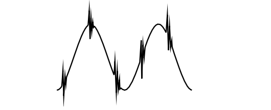
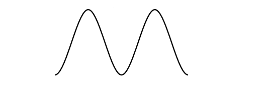
The figure shows a simple time signal which contains a sinusoidal component at a low frequency and vibrational shocks that are at high frequencies. If we set the frequency measurement that the low frequency is passed through and the high frequency is filtered out (LowPass filtering), then we will measure a signal that looks like this:

If we filter out the low frequencies and pass the shocks (HighPass filtering), then we will measure a signal that looks like this:

To remove high frequencies, we set e.g. Fmin=10 Hz and Fmax=500 Hz. To remove low frequencies, we set e.g. Fmin=5000 Hz and Fmax=25000 Hz.

We have already talked about the time signal in detail. When we look at it, we see the vibrations in time. So, there is time on the X-axis.

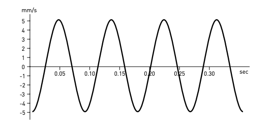
We can look at vibrations in another way. The second way is to calculate the frequency spectrum. The X-axis of the spectrum is not time but it is frequency. The spectrum itself shows us at which frequencies the vibrations are emitting energy i.e. at which frequencies the vibrations are and how strong they are, and at which frequencies they are negligible.

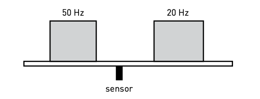
For example, two electric motors are mounted on a common frame. The speed of the first one is 3000 RPM (50 Hz) and the speed of the second one is 1200 RPM (20 Hz). We place a sensor on the frame below the motors and measure the RMS vibration value in the 10-1000 Hz band. We run just the first motor. The measured value is 8 mm/s _RMS. Now we stop the first motor and run the second motor. We now measure a value of 4 mm/s _RMS. Now we run both motors together. We measure the vibration value, which is almost 9 mm/s _RMS (exactly 8.94 mm/s _RMS).

If we only know this value of 9 mm/s _RMS, we cannot split it into two components corresponding to the individual motors running separately. So, we don‘t know what are the conditions of the individual motors. However, if we convert the time signal into a spectrum, we can distinguish the individual components.

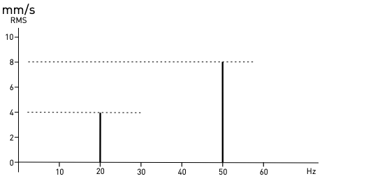
We can see two spectral lines at 50 Hz and 20 Hz. The amplitude at 50 Hz is 8 mm/s and the amplitude at 20 Hz is 4 mm/s. The spectrum thus gives us a new view of the vibration content that the time signal did not allow us to see.

The different faults on the machines differ from each other specifically in the frequency image. The spectrum thus becomes a powerful tool in vibration analysis. In the evaluation we look for high values, i.e. high spectral lines, and we are looking for the fault that causes them.

Using a few examples, we will show how easy it is to distinguish mechanical faults if we have a spectrum available.

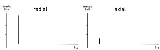
The high amplitude is only at the speed line. If it is higher in the radial direction than in the axial direction, then it is an unbalance.

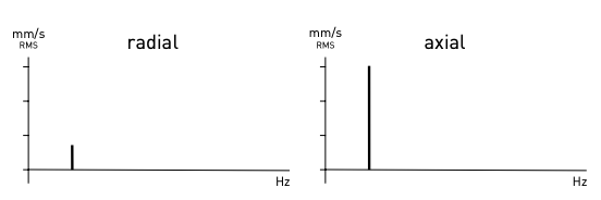
If the speed line is higher in the axial direction, then it is misalignment

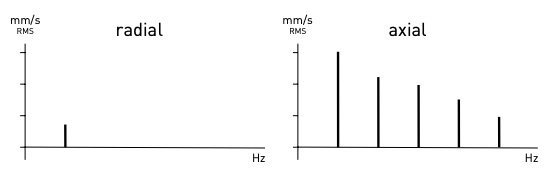
If there are also lines at multiples of speed (these are called harmonics), then there is a significant misalignment. We are still talking about the case where the axial vibration is higher than the radial vibration.

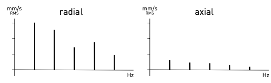
If harmonic components are present and the vibration is stronger in the radial direction, then it is looseness.

Each measurement of anything must have its physical unit. For example, mass is measured in kilograms, time is measured in seconds. The physical units used in different parts of the world may differ. To achieve some compatibility, the international SI system of units has been introduced on the principle of ensuring the same values for measuring quantities regardless of where in the world they are measured. The basic SI units include the second (s, sec, unit of time), meter (m, unit of length), kilogram (kg, unit of mass) and others.

This part will be a bit more challenging to understand.

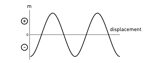
Let‘s go back to the example of the spring and the mass which we put the pen on. The pen then draws a waveform of vibrations on the moving paper. But what‘s the unit of the graph? If we want to measure any process, we always need to define its physical unit. What is the unit of mass vibration on a spring? It is obvious that the pen draws the position of the mass over time. Or we can say that it is displacement of the mass over time.

The SI unit for displacement is the meter (m). It can also be converted to cm, mm, μm, inch or milli inch (1 mil = 0.001 inch).

If the weight is moving upwards, we will refer to this direction as plus (positive). The downwards direction will be referred to as minus (negative). We assume that the values at the top are positive and the values at the bottom are negative.

We can also measure another quantities. The mass moves up and down repeatedly. We can mount a tachometer on the mass. It works like a tachometer in a car. Now we can measure the velocity of mass movement. Our tachometer has zero in the middle. The needle can deviate to the right (positive direction) or left (negative direction). It depends on whether the mass is moving up (that‘s the plus direction) or down (that‘s the minus direction). If such a tachometer would be in a car, then it would show both speeds – forward and backward.

It is clear, in the case of a spring, the speed will also change - it will not be stable. When will the speed be the greatest? That‘s also clear, the mass moves fastest when it passes through the middle position. And when will it be smallest? It will not only be the smallest; it will be zero. It will be when it reaches the maximum or minimum position. It‘s easy to imagine. At these extreme positions, the mass comes to a complete stop because it needs to change direction.

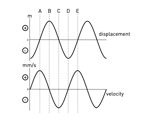
So, it‘s not surprising that if the shape of the displacement is the sine function, then the shape of the velocity will also be the sine function. In the figure, we can see the displacement waveform and below it the velocity waveform. We can see that the velocity waveform is shifted to the left. It‘s exactly a quarter of a period. If the period length is T, then the shift will be T/4 to the left, back in time.

We could also say that the velocity waveform is shifted 3/4*T to the right. This is also true. We can count the displacement in both directions because the motion is periodically repeated.

What would be the physical unit? It is velocity, so the SI unit is m/s. But for vibrations, we would get very small values in m/s. In practice we use mm/s or inch/s.

The figure shows time positions A, B, C, D, E. In position A the weight is moving (plus direction), just passing through the middle position and has maximum positive velocity

After leaving position A, the mass approaches position B. Its displacement from the center position increases. The velocity is positive, because it is upward movement. But the velocity gradually decreases as the movement stops at position B. Now the velocity is zero, the positive displacement reaches the maximum value.

After leaving position B, the mass approaches position C, where it passes through the middle position. From B to C the velocity increases in the negative direction (the mass is moving down). At point C the negative velocity is the highest.

After position C, the mass approaches position D, which is the maximum negative displacement (downward). The negative velocity decreases. The mass reverses the direction of motion in D, where the velocity is zero.

After leaving position D the mass moves upwards so the velocity is positive. The mass reaches the middle position E and the process repeats. The position E is equal to A.

As far as the velocity values are concerned, they are positive (plus) when the mass is moving upwards (we have marked this movement as plus). The velocity values are negative (minus) when the mass is moving down.

The last quantity used is acceleration. The physical nature of acceleration is change of velocity. If a rock is falling, it is falling faster and faster because of the gravity force. And that‘s a very good example. For an object to accelerate or decelerate, a force must be acting on it. To accelerate a car, the force of the engine must be acting (that is, positive acceleration in the direction of velocity, i.e., in the direction of motion). In the opposite case, to decelerate, the force of the brakes must act (this is a negative acceleration against the direction of speed, i.e., the direction of motion).

Also, our mass on the spring is exposed to the force generated by the spring. If we compress the spring, then the spring creates a force against the compression and tries to get back to the central position. However, when mass comes to the central position, the movement does not stop. The inertia causes the mass to move continuously through the middle position. It starts to stretch the spring. The stretched spring creates a force in the opposite direction. It wants to get the mass back to the middle position. This process is repeated.

The force is really the equivalent of acceleration. The formula F= m*a describes a relation between mass, force, and acceleration. Because mass m is constant, then we can see that acceleration is directly related to the force.

In next figure we can see the displacement and the acceleration. We can see that the acceleration waveform is shifted half of period to the left. Comparing it with the velocity waveform, we can see that the acceleration waveform is shifted a quarter of a period to the left or back in time. Not surprisingly, the acceleration waveform again corresponds to the sine function.

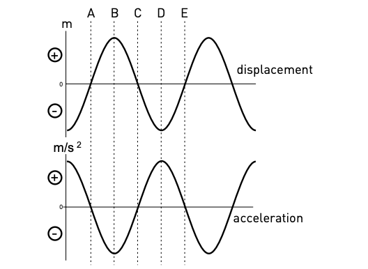
The understandings in this case are a little more complicated, but let‘s get into it. Let‘s describe each position A to E and the processes in between.

A
The mass passes through the middle position with maximum velocity. Velocity was increasing before A and will decrease after A. It is the middle position, the spring is not compressed or stretched. There is no force acting at A point. So, the acceleration is zero. If we want to imagine the position of A in a car, then before A we press the accelerator and accelerate. At A we move our foot from the accelerator to the brake and after A we press the brake and decelerate

A - B
The inertia moves the mass up and compresses the spring. The spring generates a downward force, and the force is greater the more it is compressed. The movement of the mass is positive (upward movement), the acceleration (i.e. force) is negative (i.e. against the movement). The movement of the mass is slowed down.

B
The force of the compressed spring stopped the upward movement. The mass changes movement direction to negative (down), the velocity is zero. However, the spring is still compressed and generates a negative (downward) force that initiates the downward motion of the mass.

B - C
The force of the compressed spring keeps pushing the mass down and accelerates its movement (negative direction). However, this force gradually decreases. The less compressed spring generates less force. The mass therefore accelerates less, but still downwards.

C
The mass passes through the middle position. This is the neutral state of the spring, when it is neither compressed nor stretched and does not generate any force. The acceleration is zero.

C - D
Inertia keeps the mass moving downwards (negative) and the spring stretches. It generates an upward force against the downward movement. Now we have a battle between inertia and spring resistance. The force generated by the spring keeps reducing the inertia until it cancels it out completely. It wants to return the mass to the middle position.

D
The force of the extended spring stopped the downward movement. The velocity is zero, the direction of motion changes to positive. The stretched spring still generates a positive force upwards and the mass starts to move upwards as well.

D - E
The mass accelerates upwards.

E
Here, the entire period of movement is completed. The inertia force starts to contract the spring. We have reached the same situation as in position A.

In the description of the displacement, velocity, and acceleration, we needed to express the shift of one signal with relation to the other. Such a shift is called a phase shift. We have used expressions such as quarter period or half period. The shift could be defined in time (in seconds). But this has the disadvantage because the period time of different frequencies is different. In practice, therefore, a different approach is used..

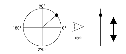
Imagine that we have a ball tied to a string and we are swinging it in a circle. Looking from the front, we see that the ball is circling around the center. But looking from the side, we see the ball vibrating between two extreme positions. It looks just like a mass on a spring. When we measure the waveform of this motion, we again get a shape corresponding to the sine function.

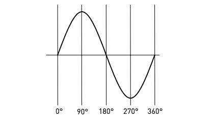
This approach allows us to imagine one period as an angular value. The ball goes around the circle once during one period. And the circle has 360 degrees. So, the length of one period can also be thought of as 360 degrees. The advantage of this approach is that it doesn‘t depend on frequency. So, it doesn‘t matter how long one period lasts in seconds. Angularly, it simply always lasts 360 degrees. If we then want to say that the velocity waveform is shifted by a quarter of a period to the left (i.e., against time), then we say that it is shifted by minus 90 degrees. 90 is a quarter of 360 and the minus sign represents the direction against time.

So now we know that the phase shift is in degrees.

Vibration diagnostics has two basic tasks in practice. The first is to determine the machine condition has been changed. This is called problem detection. The second is to analyze the vibration in more depth and find out what fault or wear has occurred on the machine.

Detection measurements need to be simple and quick so that we can measure machines as often as possible. Overall measurements are used the most. The meaning of the word overall is that the measurement covers a wide band of frequencies. The measured value can then be RMS (which is the most used), 0-P, P-P and others.

If we want to tell someone what overall value we have measured, we always have to tell them four parameters. If we say we measured 4.8, it‘s completely worthless. If we add a unit and it‘s 4.8 mm/s, it‘s a bit better. We also need to add information about what type of calculation we used (e.g. RMS). So, we get 4.8 mm/s _RMS. And the fourth information is what frequency band we measured in, i.e. what bandpass filter was used (e.g. 10-1000 Hz).

So, the correct expression is 4.8 mm/s _RMS in the 10-1000 Hz band.

Always remember this rule of four.

If the type of calculation is sometimes not mentioned in the text or in the graphs, then it does not matter whether we measure RMS or 0-P.

If we know that we can measure the displacement, velocity, and acceleration of vibrations, we should also say with what we measure in practice. In most cases, acceleration sensors are used for measurements. They are affordable and can measure in a wide frequency range. The advantage is that we can convert the acceleration signal into velocity and displacement quite easily.

There are some complications for very low and very high frequencies, but we will discuss that later.

To measure machine vibrations accurately, the sensor must be mounted on the machine properly. Firstly, we must ensure repeatability of the measurement. This means that we must always measure in the same place and the sensor must always be mounted in the same way. In no case we can hold the sensor in our hand and just press it to the surface of the machine. The mounting method mainly affects measurements at high frequencies. In practice, mounting with a magnet is used. But the magnet cannot just be pressed to the surface of the machine. It is not flat and the sensor could swing during measurement. This would destroy the measured value. We would not be able to repeat the measurement and measure the same value. That is why measuring pads are glued to the machine. They are stainless steel, magnetic and have a completely flat surface. The sensor with the magnet then holds perfectly on the pad. Repeatability of the measurement is ensured. It is also ensured that we always measure in the same place.

First, we explain what the radial and axial measurement direction is, it means in which direction we mount the sensor on the machine.The radial direction is the direction perpendicular to the axis of rotation, i.e. perpendicular to the shaft. With a horizontal shaft it is quite indifferent whether it is mounted vertically, horizontally or diagonally. On the vertical shaft it has no effect.

The axial direction is the direction parallel to the axis of rotation, i.e. parallel to the shaft.

To measure the bearing condition, we need to place the sensor close to the bearing. It does not matter in which direction. Usually, radial directions are used.

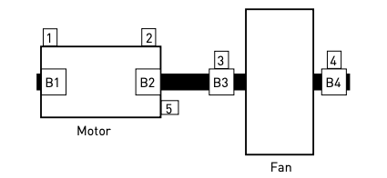
The picture shows a typical machine setup, which consists of a motor and a fan. We have 4 bearings marked B1 to B4. For each bearing we measure radially (sensors 1 to 4) and once on the machine axially (sensor 5).

The speed is measured by a speed sensor. We call it a tacho probe. This probe shines a laser beam that we point at the rotating shaft. We place a small reflective tape on the shaft. Now we connect the tacho probe to the analyzer and it receives the reflections from the shaft. When the beam reflects off the tape, the tacho sends a voltage pulse. Then analyzer measures the time T (it‘s actually the period of rotation) between the pulses and can calculate the speed as 1/T.

We always start with overall RMS values. Don‘t think this is something less. We can do vibration diagnostics with them with excellent results. We can add more sophisticated methods later. There is no point in using procedures that we don‘t fully understand. But it is also a common misconception that vibration diagnostics is something as easy as measuring temperature or pressure. That all it takes is a day‘s training to make us an expert. One day‘s training will show us how to get started easily so that we have results immediately. Then we will take a long time to develop and gradually understand even more complex procedures. Being an expert in vibration diagnostics will ensure that you will always find employment very easily because you will know something that others do not. And every factory wants to know the condition of its machines and prevent unexpected breakdowns.

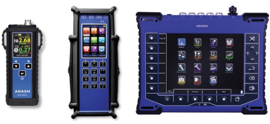
If you use Adash vibration analyzers, you will find both – basic measurements with preset parameters and advanced measurements where you can set all the parameters according to your requirements.

There are two basic groups of machine faults. The first are mechanical failures.

Unbalance – when the rotating rotor has a heavy point, this mass creates a centrifugal force and it shakes the machine. It is the same as an unbalanced wheel on a car.

Looseness – the machine is fixed to the base with bolts, if any of them has lost rigidity or even breaks then the fault is looseness.

Misalignment – for example the motor is connected to the pump by a clutch. If their axes are not in a straight line, then we are talking about misalignment.

We measure values in velocity for mechanical faults, in RMS and usually in the band from 10 Hz to 1000 Hz. If the speed is lower than 10 Hz (i.e. 600 RPM), then we measure from e.g. 2 Hz.

The second group includes rolling bearing wear, gearbox gearing defects, etc. Here we make measurements in acceleration, in RMS and usually in the 500 Hz band up to the maximum range of the analyzer. This is usually 25 kHz. Acceleration is most often measured in g, which is the value of the acceleration due to gravity. 1 g = 9.81 m/s², where m/s² is the SI unit. If g has to be converted to m/s², then feel free to multiply by ten.

We have measured the first values. What do we do now?

There are standards for mechanical faults that give limit values for good condition, warning and danger. If the warning limit is exceeded, the machine can be still operated, but repairs must be scheduled. We should also measure the machine more frequently, as an already present fault can get rapidly worse. Exceeding the danger limit should mean shutting down the machine and having it repaired or adjusted.

The most used standard is ISO 20816, which contains several categories of machines and specifies their vibration limits. It uses the velocity measurement of vibration to detect mechanical faults.

Unfortunately, there are no standards for the bearings condition. Commonly used limits tend to be around 1 g _RMS for the warning limit and 2 g _RMS for the danger limit. We only measure higher frequencies, usually Fmin=500 Hz.

If we have several machines of the same type, then we can compare the values between these machines. For example, if we measure 1.5, 1.7, 1.4, 5.6 and 1.3 mm/s _RMS on five machines, then it is clear that machine 4 with a value of 5.6 is not OK.

If we have already measured several values at one place, e.g. one week apart, then we can see the trend. And we use the following rules: If the values are more or less the same in the trend (± 15%), then the machine is running in a stable condition and we do not repair anything on it. If the values are rising, then there is a fault and we must deal with it.

If we have stable values in the trend at the beginning, then we take them as a reference. Then we can set the warning limit to twice the reference and the danger limit to five times the reference.

Watch the speed!

If the machine is always running at the same speed, then measured values are not affected by the speed. But watch out for machines that change speed. The measurement value also changes when the speed changes even if the machine condition is the same. In the case of, e.g. unbalance, the centrifugal force increases as the speed increases and thus the vibration value increases. It is the same with bearing wear. If pitting is present on the rings over which the balls roll, then again at higher speeds the vibration value will increase. Therefore, the speed value should always be stored with measurement value on such machines. Either we can measure them with a tacho probe and the analyzer will store the speed with measurement value, or we can enter the speed manually before measurement, or we can add speed in the computer later.

Even with a simple instrument, very reliable diagnostics can be performed. An example of such an instrument is the Adash 4900 Vibrio.

It can measure more than just overall values, but we will not talk about advanced features now. The basic measurement is a velocity measurement in the 10-1000 Hz band. The method of evaluation is RMS, so if we want to write a value in a report, then for example we write 4.8 mm/s_RMS 10-1000 Hz. The second measurement is the acceleration measurement in the 500-16000 Hz band. The method is again RMS. So, we will write e.g. 1.7 g _RMS 0.5-16 kHz.

We start by the acceleration measurement. The most common use is to measure the bearing condition. Low values up to about 0,3 g _RMS always mean excellent condition. We are talking about standard bearing types that operate at 600-3600 RPM. For lower speed, even a value of 0,3 g _RMS can indicate wear. On the other hand, for higher speed, the value can reach even higher values although the bearing condition is good.

The use of vibration velocity values is a bit more complicated. We are looking for the mechanical faults which were already described, such as unbalance, looseness, and misalignment.

If we have measured higher values either according to the standard or according to our experience, then we can use following criteria:

a) Misalignment detection. If the vibrations in the axial direction are higher than in the radial directions, then misalignment is the most likely fault. We should align the machine and measure again.

b) Looseness detection. If a) does not apply, then we measure the vibrations at all the mounting bolts of the machine. If there is a higher vibration value on one bolt than on the others, then there is a looseness. It may just be a loose bolt or the bolt may already be damaged. We measure again after the repair. We do not need to have measurement pads on the bolts for this measurement. It is just a comparison of the values. Just placing a magnet next on the machine foot is enough.

c) Unbalance detection. If neither conditions (a) nor (b) are met then it is most likely an unbalance. Again, after balancing, measure the values again.

There may be situations where the vibration remains high after repair or adjustment. Then there are problems that have not yet been mentioned, such as resonance or electrical unbalance.

Many of you know the concept of critical speed. This concept is especially important on lightweight large machines such as a turbine. But the problem also occurs on ordinary machines. Let's imagine that we increase the speed of the machine and at the same time we measure the value of the vibration velocity in the 10-1000 Hz band. It is normal that as the speed increases, the vibration value gradually increases. However, there may be a situation where the vibration value increases rapidly by a large value. For example, a relatively small change in speed from 1300 RPM to 1400 RPM will cause the vibration amplitude to double. This is no longer normal. If we increase the RPM further, the vibration drops again. It is an unexpected paradox. The vibration curve is shown in the picture

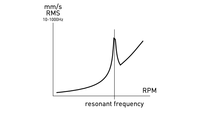
The speed is on the X-axis and vibration value is on the Y-axis. The frequency of the peak is called the resonant frequency. This is a mechanical characteristic of the machine. At resonant speed the unbalance centrifugal force suddenly builds up a much higher vibration value. This speed is called critical speed and the machine should not be operated at this speed value under any circumstances. What concerns us in practice, however, is not the resonant frequency of the machine itself. The machine manufacturer pays attention to this and the first critical speed must be higher than the operating speed used. This is not valid for turbines, for example.

So, the machine itself is fine. What can cause a resonance problem?

The answer is simple. Poor mounting frame design may be the cause. If the machine is mounted directly on a heavy concrete foundation, then resonance is not a problem. But if the machine is mounted on a steel frame which is supported only by concrete blocks at each end, then resonance can easily occur. The frame may be poorly designed as it is too flexible and the problem will appear.

Each frame has its own resonant frequencies. We are usually interested of the first i.e. lowest one. If the speed is close to first resonance, the frame is deformed. It's the same as a string on a guitar that vibrates at its first resonant frequency. You can even see with the eye how the string deforms.

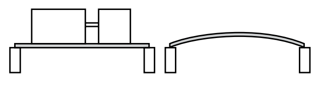
We can detect the problem in different ways when we use the measurement:

a) If the speed of the machine can be changed (Variable-frequency drive is used), then we start at a low speed and gradually increase it. At the same time, we measure the vibration velocity in mm/s RMS 10-1000 Hz. If the vibration suddenly increases at a certain speed and then drops again, the problem is the resonance of the frame at that frequency = speed.

b) If the speed cannot be changed, then we run the machine at operating speed. We start continuous measurement. The vibrations are high. We turn off the power and look at the vibration values during coast down. If there is a significant sudden decrease, then it is suspected that the operating speed is close to the resonance frequency.

c) If the speed cannot be changed, then we run the machine at operating speed and we take measurements at several points on the frame.

We draw the measured values into the picture.

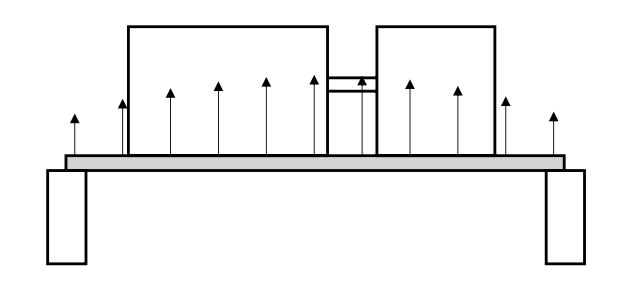
If there is frame deformation at the resonant frequency, then the values should show low values at the edges where are the supports and highest in the middle.

You need to change the frame or change its mounting to fix this problem. Adding another support in the middle will always help.

In the case of electric motors, there may be a situation where the electrical winding is not in good condition. It may be interrupted or short-circuited in several places. The electromagnetic forces are not balanced then and they move the rotor away from the center of mass, i.e. from position where it should properly be located. It looks like an unbalance. But rebalancing of the rotor does not bring any major improvement.

This fault can be detected by a simple test. We place a sensor to the motor and start a continuous measurement of the RMS vibration velocity in the 10-1000 Hz band. This means that we see a new measurement value on the display approximately every second. Now we turn off the power to the motor. It will start to slow down and stop after some time. Two situations can occur:

a) When the powering is switched off, the vibration slowly decreases until the engine stops.

b) The vibration increases for a very short moment after the powering is turned off and then drops immediately to almost zero.

We can see the described examples in the pictures on the next page

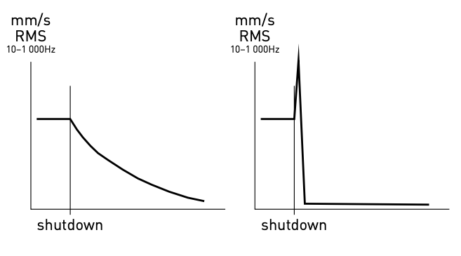
On the left, there is a case of slow vibration decreasing, which means that the rotor is indeed unbalanced. Thus, there is a heavy spot.

On the right, there is a case of sudden drop. This means that the whole vibration problem is related to the failure of the stator and rotor electrical windings.

The more inquisitive among you will now ask what the peak in the second case means. The answer is simple. When the power was turned off, the electromagnetic forces disappeared. They deflected the rotor from its proper position in the center of mass. Thus, a mechanical shock occurred when the rotor returned to the center of mass. This caused an increase in vibration. The next values are very low because the rotor is not mechanically unbalanced.

Firstly, we need to create a structure of the factory. This means creating a list of machines that we will measure. Then we create a list of measurement points for each machine. For these lists we use the programs that we buy together with the measuring instruments. For example, Adash offers the DDS program.

We create the entire structure of the company in that program. We can create several levels like Hall 1, Section 3, and a list of machines. Then we create measurement points on each machine and the required measurements on them. Then we transfer this list to the analyzer and we can start measuring. When we are in the field, we just select from the list which machine and which point we will measure.

We don't have to set anything up in the field. Everything in analyzer is set up automatically according to the measurement definition created in the computer program in advance.

The transferred list is called a route. It determines where we will go and measure.

When we return from the route, we transfer all measurements to the computer and we can start evaluating them.

The DDS program contains many tools to automate, speed up and simplify the evaluation.

How often should we go for the route? Probably the optimal time is two weeks. If our company is large, it may be at longer intervals. The maximum interval that should not be exceeded is 2 months.

What to watch out for? We cannot make many mistakes when we go for a route. We have defined the parameters in advance in the computer. The only real danger is that we may measure in the wrong measurement point or even on the wrong machine. The data will then be stored in the computer to the wrong place. We will be confused during data evaluation, how the new data is so dissimilar to the previous measurement.

Our evaluation ends with the creation of a report to maintenance department with actions they should take. We should always keep in mind that maintenance personnel do not understand the concepts of vibration diagnostics very well. Therefore, let's not even bother them with it. We should use a vocabulary they understand. We keep reports as short as possible. There is no need to include a long list of machines that are in good condition. Only machines which need an adjustment or repair should be included in the report. Maintenance prefers a report with only a brief statement: EVERYTHING IS OK.

It is absolutely the best if a company purchases vibration diagnostic equipment and has its own employees to perform the measurements and their evaluation. This is because they are in constant contact with the machinery and get information from maintenance about which repairs or even replacements have been made.

It is also possible to purchase vibration diagnostics externally as a service. This solution has several disadvantages. The external staff only comes in at defined time intervals and measures the route. They usually do not know anything about maintenance interventions between the routes. Their approach is quite different. They measure a lot of companies like yours. You have no equipment to take measurements yourself if necessary. It may be too late to measure during the next visit of an external analyst. But if you do decide to go with an external company, then we make a few recommendations.

If an external company comes to you with an offer of measurements, always take them to the machine. Let them take the measurements and give their opinion on the results. Don't waste your time with a person who makes the excuse that he is only making the offer and others perform the measurements. It is always positive when the person offering the measurement already comes dressed in work overalls. Never be fooled by the claim that the whole vibration diagnostics thing is very complicated and cannot be understood by the customer.

There are also solutions where you measure the routes yourself and send the data only for evaluation. You are always told that a team of experts is available to evaluate the data. The question is how many of them have ever been in the factory. I heard a good comment from an experienced diagnostician who has been measuring in the business for many years. He said, "I wouldn't take a recommendation for a repair from a guy I've never seen. And who, moreover, has never seen my machine." That's an exact definition of how to approach to these services. You will never be able to include in a contract with an external company their financial responsibility for failing to detect a fault or reporting a fault that does not exist.

And what about artificial intelligence? At Adash, we have tried to use AI several times. The first time was around the year 2000. I can responsibly say that it will not be applicable in vibration diagnostics. The reason is simple; there will never be a training set that contains enough measurement results on many types of machines.

If I compare it to medicine, how could an artificial intelligence work if it should diagnose diseases not only for humans but also for animals? Because humans are just one type of organism, therefore one type of machine. And there is a huge number of types of machines in diagnostic practice.

So, always be very suspicious and don't be afraid to ask many questions when you are evaluating potential offers for external diagnostics.

Today, it is mostly just a bureaucratic matter for the various quality systems and their audits. In modern instruments there are no setting elements to adjust the measured values in the calibration laboratory according to the standard.

If we have only one instrument and we want to check that it is measuring correctly, then a calibration lab makes sense. However, there are also electronic instruments that simulate a sensor. They generate exact voltage values. We connect them to the instrument and check if the instrument shows the correct value.

If we have more than one instrument and more than one sensor, we can switch between them during the checks. If something is wrong, we can easily find out what it is. It could be a sensor, a cable, or an instrument.

What is rolling bearing wear? It is the wear of the tracks on which the balls or rollers roll and the wear of the surface of the balls or rollers themselves. This wear is called pitting.

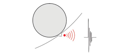
What happens when the ball hits a fault (hole) in the bearing track?

There will be a shock. It's like hitting a bearing with a hammer. As one ball after another hits the hole, a time signal containing individual shocks is produced.

If we know the speed and dimensions of the bearing, then we can calculate how far apart the shocks will be. So how far apart in time they come. And now the magic comes. If a hole appears on the outer ring, inner ring, on the ball or the cage is cracked then the time interval between shocks is different. It means we can distinguish them.

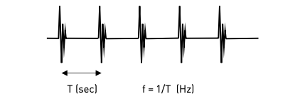
If the shocks come at a regular time interval, then we can calculate the frequency. That is, how many times a shock comes in one second.

And since the time interval varies for different defects, so does the frequency. These frequencies are called bearing fault frequencies. And the spectrum allows us to look for them.

There are four fault frequencies:

BPFO – Ball Pass Frequency Outer
BPFI – Ball Pass Frequency Inner
BSF – Ball Spin Frequency
FTF – Fundamental Train Frequency

The frequencies of shocks are high. Therefore, the acceleration signal must always be measured. It measures high frequencies well.

But the situation is not quite that simple. We can calculate the spectrum directly from a time signal with shocks. But no amplitudes at the fault frequencies are visible. Although there are significant peaks in the time signal (2 g), the peak value in the spectrum is 0.0008 g RMS.

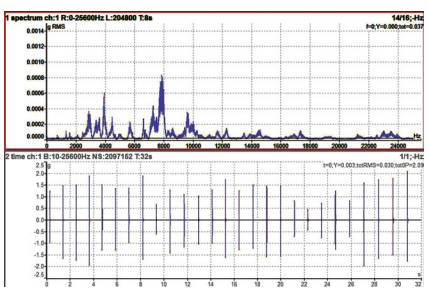
The reason is as follows. The height of the lines in the spectrum corresponds to the RMS values. And this corresponds to the energy contained in the signal. Recall the explanation of the RMS value and the filled areas. The spectrum only responds well to significant areas in the signal. It does not respond well to high peak values without significant area under the signal.

So now we know why we can't calculate the spectrum directly from the measured signal. We have to do something with it first. We have to add some significant areas. The first step is to filter out the low frequencies.

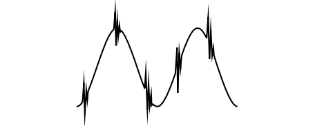
. We've got shocks but we also have a sinusoidal waveform at the speed frequency. We don't want that in the signal. That's why we filter out everything below 500 Hz first.

Now we will pass the signal to the envelope modulator. This will add a significant area to the signal.

The individual shocks are converted by a diode (which passes only positive voltage), then it charges capacitor C and then it is slowly discharged through resistor R. This produces a signal at the output similar to the shock envelopes.

The spectrum calculation responds much better to this signal and we can see significant peaks.

If the fault is only on the outer ring, then we can see its frequency (BPFO) in the spectrum, followed by its harmonic components.

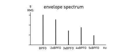
Now I will explain why the harmonics are in the signal. If we calculate a spectrum from a signal where there is only a sine wave at frequency f, then (given certain other conditions) there will be only one distinct line at frequency f in the spectrum.

However, if the time signal is, for example, rectangular, then the spectrum will contain a frequency f and many harmonics. And this is true for all signal shapes that are not sinusoidal. The spectrum always responds to signal distortion by showing harmonic components. And an envelope signal is a highly distorted signal. It's far from sinusoidal.

The advantage of demodulation is that we can detect a bearing fault at a very early stage. Another advantage of knowing the fault frequencies is that we are not confused by other frequencies. They may be in the spectrum and have nothing to do with the bearing fault (e.g. shocks caused by gear tooth wear).

We now describe a common misunderstanding of the demodulation process. Bearing fault frequencies can be very low. The user asks whether he must use a sensor that can measure such low frequencies. The complete opposite is true. The defect lines in the spectrum are created by calculation, not by measurement. We need to have shocks in the measurement and then convert the time interval between the shocks to frequency. Nothing is measured at the fault frequencies! If we would have an accelerometer that measures from 500 Hz upwards, then we can use it. After all, we remove all frequencies below 500 Hz before envelope modulation anyway.

Fault frequencies allow us to deal with situations where we have two different bearings side by side. We can clearly see in the spectrum which one is damaged and needs to be replaced.

This is an old method of vibration evaluation. A screwdriver was pressed face down on the machine and the back surface pressed against the ear.

Even today, our Adash instruments allow us to listen to vibrations. The signal from the sensor is fed into the headphones. The bearings (their noise or whistling) are most often listened to. Various repetitive phenomena, various knocking inside the machine can be heard well. Of course, you cannot listen to the signal from mechanical faults. It means, we do not hear them, our ear is not sensitive at such low frequencies and the headphones transmit them with great attenuation.

Ultrasound is a signal at frequencies higher than 25 kHz. There are special microphones that can pick up such high frequencies. They are most sensitive at frequencies around 40 kHz. They can be used to measure bearings, but do not offer any advantages over acceleration sensor measurements. They are useful in finding leaks in pressure distribution.

Adash vibration analyzers also allow this measurement.

To perform such a recalculation simply by multiplying by a constant, it is necessary that the signal has to have a sinusoidal shape. If it is not, the recalculation cannot be performed simply. Mathematically, of course, it is possible, but we have to know how to use derivatives and integrals.

So, let's have an acceleration signal with some RMS value or 0-P. Just a reminder that 0-P=RMS/0.71. The frequency of the sine wave is f. Then the velocity values are equal:

vel_RMS = acc_RMS / (2·π·f)      vel_0-P = acc_0-P / (2·π·f)

Then the following formulae apply to the displacement:

disp_RMS = vel_RMS / (2·π·f)      disp_0-P = vel_0-P / (2·π·f)

Once again, keep in mind the sine wave condition.

The best way to understand this is through examples. Consider two machines that exhibit different vibration values.

A) The machine operates at a very low speed of 300 RPM (5 Hz) and the displacement RMS value is 100 μm.

B) The high-speed turbo compressor operates at 120,000 RPM, which is 2,000 Hz and the acceleration RMS value is 1 g.

If we measure machine A with a displacement sensor that has a sensitivity of 8 mV/μm, then for a value of 100 μm we get 800 mV. An electrical signal with amplitude of 800 mV is very easy to measure. Now let's try to measure machine A with an acceleration sensor. Firstly, let's calculate what acceleration value is on machine A. From the above formulae, we can see that:

acc_RMS = disp_RMS · (2·π·f)²

Fill in the numbers:

acc_RMS = 100 μm · (2·π·5)² = 100 μm · (31.4)² = 100 μm · 900 = 90 000 μm/s² = 90 mm/s² = 0.09 m/s² = 0.009 g RMS

The value of 0.009 g is difficult to measure. With sensor sensitivity 100 mV/g, this is a value of 0.9 mV, which may already be hidden in noise.

If we measure machine B with an acceleration sensor that has a sensitivity of 100 mV/g, then for a value of 1 g we get 100 mV, which is easy to measure.

What happens if we try to measure machine B with a displacement sensor. The formula is:

disp_RMS = acc_RMS / (2·π·f)²

Fill in the numbers:

disp_RMS = 1 g / (2·π·2000)² = 10 m/s² / (12 000)² = 10 m/s² / 144 000 000 = 6.9·10⁻⁸ m = 0.000 069 mm = 0.069 μm

With a sensor sensitivity of 8 mV/μm we would get 0.5 mV, which is very low and may already be covered by noise. So, measuring the B machine with a displacement sensor would not be a good idea either.

Similarly, calculate what the displacement value would have to be at 1 Hz when acceleration value is 3 g. If you came up with an RMS value of 0.76 m, then you calculated correctly. The RMS of 0.76 m_RMS is approximately 1 m 0-P. It means that the machine would vibrate +/- 1 m around the center position. I just wanted to show that higher acceleration values at low frequencies are impossible, because there would have to be huge displacement values. Likewise, higher values of displacement at high frequencies are impossible because there would have to be huge values of acceleration.

So far, we have only talked about measurements with a portable vibration analyzer. But there are also instruments that measure continuously. It means that sensors are mounted on the machine and the machine condition is monitored continuously. It has the advantage that you can monitor the condition continuously and catch a problem immediately. Continuous measurement means that, for example, we measure a new vibration value every second. In the route measurement method, we obtain a new value e.g. once in every two weeks.

Of course, you have to pay for this advantage. The prices of online systems are higher than portable systems prices. While one portable analyzer is sufficient for routes, we need one online system for each machine.

There are two basic facts to remember when you set up an online system:

1) the processor performance is not infinite
2) the disk capacity for data storing is not infinite

Although both statements are clear and no one is questioning them, you'd be surprised how many users forget them when they are setting up their online system. They don't calculate how much disk space they use in a day, for example.

Systems in the past have not measured completely continuously. The user set how often the value should be measured, e.g. every 10 minutes.

Current Adash systems measure continuously. During the development process, we also put a lot of effort into developing algorithms to handle large amounts of data.

The basic idea is this: it makes no sense to save measurement values that don't change. If the value is equal to 3 mm/s then it is sufficient to store it e.g. once every hour or even more hours. Of course, when you look into the graphs, you know that a gap of 3 hours between measurements does not mean that a measurement was taken once in every 3 hours. You know that it was measured all the time and that the value was stable. The Adash storage algorithms use this approach for all types of measurements. The user must not miss any data that signifies a change of a machine condition.

Data reduction also means faster access to data in the database and faster display of trends.

Vibration measurement also makes balancing of rotors very easy. We won't go into too much detail. In practice, rotors with one or two balancing planes are operationally balanced. Single-plane balancing is performed on narrow rotors where the radius is significantly larger than the width. Two-plane balancing is performed on rotors which are wider. We see two-plane balancing in practice in the balancing of car wheels. One weight is put inside and the other is put on the outside.

We describe the case of one plane, which is simpler. We connect a sensor to the rotor bearing and a tacho probe to measure the speed. Tacho probe is important because we will only be measuring amplitude and phase at speed frequency. In Adash instruments this measurement is called amp+phase measurement.

We spin the rotor to operating speed and measure the initial values. Then we mount a trial mass to the rotor. Its weight is recommended to be about five times the value of the permissible allowable residual unbalance (every rotor is always a little unbalanced, the term permissible allowable unbalance means the value where we do not have to balance and can operate the machine without limitations). Then we spin the rotor again and measure the trial run amplitude and phase values. Now the analyzer calculates how heavy mass is needed and where it should be placed. The position of the balancing mass is read from the reflective mark on the shaft, which is used by the tacho probe. It is in degrees and the full circle of the rotor is 360°.

Balancing in two planes is similar, but more measurements are taken. The trial weights must be placed successively in the first and then in the second plane. The results are two weights and two positions. One for each plane.

It is a good idea to test the balancing process first in the office, e.g. on a desktop fan. The unbalance can be simulated e.g. with plasticine. The final balancing weight should have the same weight and position opposite the simulation plasticine.

For balancing, the ISO 1940 standard is used, which describes both the procedures and the recommended permissible residual unbalance for different types of machines and different speed values.

Sensor settings

ICP on/off – Most sensors contain internal electronics that require a power supply, which is called ICP® (PCB Registered Trademark). If the sensor does not require power and we leave the ICP power on, then we can damage the sensor. If we are connecting a signal generator to the analyzer input, then always leave the ICP off.

Unit – A sensor is a device that converts a physical quantity into a voltage or current. A voltage is at the output of the vibration sensor and we have to set what physical quantity it converts to the voltage. Most often we have acceleration sensors, so we set g or m/s².

Sensitivity – Here we set the conversion factor between the unit and the output voltage, for g it is usually 100 mV/g. That is, if the signal value is 1 g then 100 mV is at the output of the sensor.

Overall measurement settings

Channel – The channel number on which we want to make the measurement.

Unit – The physical unit in which we want to make the measurement. Caution - do not confuse with the sensor unit, which is e.g. g, the instrument can convert the signal into mm/s or μm. So, for measuring the bearing condition we choose g, for measuring mechanical failures we choose mm/s.

Detect type – Choice of evaluation method. Most often we choose RMS, others are used only in special cases.

Band Fmin, Fmax – Here we set the frequencies of the bandpass filter. It removes all frequencies lower than Fmin and all frequencies higher than Fmax from the input signal. Then the value, e.g. RMS, is evaluated. It depends on which faults we are interested in. For bearing condition measurements, we choose high frequencies, e.g. 5-25.6 kHz. For slow-running bearings, we choose a lower Fmin, e.g. 500 Hz. For mechanical faults measurement we usually choose 10-1000 Hz, for slow running machines (speeds below 600 RPM, i.e. below 10 Hz) we choose Fmin e.g. 1 Hz. The lower the value, the longer you will wait for the measurement. The waiting time is necessary to settle the sensor after it has been attached to the measurement pad. For a value of 10 Hz, it is 1 second. For a value of 1 Hz, it is 10 seconds.

Samples – By setting the number of samples, we set how long measurement we want to take to calculate the result. Usually, a length of 1 s is sufficient. The measurement should always include at least 10 rotor revolutions.

Time signal measurement settings

We have explained the measurement of the time signal using the example of a spring and vibration recording. The basic parameters Channel, Unit, Band Fmin, Band Fmax, Samples have already been explained in the previous overall measurement setting.

Sampling Frequency – This value determines how the analog signal will be converted to digital. The analyzer always sets the sampling frequency itself according to the set value of Band Fmax. We do not recommend changing this value until you have a deeper understanding of the measurement.

Spectrum measurement settings

We have already explained that this is the conversion of a time signal into a spectrum. The calculation is done by FFT (fast Fourier transform). We do not need to know more about the calculation.

The parameters Channel and Unit have already been explained in the previous setting of the overall measurement value.

Window – Keep the option 'Hanning', understanding of the window function requires deeper knowledge and is not necessary to perform diagnostics.

Band Fmin – It is only the Fmin band setting. If you are not interested in frequencies below 10 Hz, then leave 10 Hz, otherwise enter a lower value. A lower value increases the measurement time, as we have already explained for the overall measurement.

Range – Setting of the Frequency range of the spectrum. Usually, 1000 Hz is enough for mm/s measurements, when measuring in g we want to see high frequencies, so we enter e.g. 25600 Hz.

Lines – This setting is the same as image resolution. High resolution allows us to zoom in on the image and see the details. When we enlarge a low-resolution image, we only see rectangles with no internal structure. It is similar with spectrum, when we have two close frequencies next to each other. If we need to separate them, we need to choose a higher resolution to allow this. The df value shown below the number of lines shows the frequency difference between the neighboring lines. If we need to resolve two frequencies that are e.g. 2 Hz apart, then the df should be at least 0.5 Hz. A higher resolution always means a longer measurement time. The measurement time is easily calculated without a calculator. We take the value of df (i.e. the distance between lines) in Hz and calculate T=1/df, T is the measurement time. For example, if you set the Range and Number of lines so that df=0.01 Hz, then the measurement will take 100 sec.

Averaging – Vibrations may not always be completely stable or may contain a lot of noise. It is a good idea to use averaging. For example, if we set a value of 8, then 8 individual measurements are taken. One arithmetic average is calculated from them and saved. The averaging value of 8 is sufficient in most cases.

Demod spectrum measurement settings

You can also find the concept envelope analysis in the literature. It is exactly the same measurement.

The parameters Channel, Window, Unit, Averaging have already been explained earlier. Demod spectra can only be measured in acceleration, so the choice of units is limited.

Warning: as explained earlier in a separate chapter, do not confuse the meaning of Demod Fmin, Fmax and the meaning of Range.

Demod Fmin, Fmax – The frequencies of the input filter, the task of this filter in demodulation is to remove the frequencies of the speed and harmonic components. Only the shocks are to remain, because only these are needed for the subsequent envelope modulation.

Range – Spectrum range after envelope application. Here we want to see the bearing fault frequencies, these are usually below 100 Hz. The range is therefore sufficient to a few hundred Hz.

Lines – No need to have many lines. The fault frequencies are quite far apart, so we don't need a high resolution. 1600 lines is perfectly sufficient.

If the measurement is careful and reliable, we can detect machine faults and malfunctions early on, which ultimately means saving time and money. It is an exaggeration to say that measurement will become your indispensable assistant.

You surely won't become a master after your first measurement, but we believe your skills will improve over time and pass this manual to new beginners.

After all, we know what we're talking about. The world of vibrations is our world. Besides, you won't be left alone in this. You will find plenty of articles, videos, and more manuals about this on our website.